
Descriptive statistics: the first thing you do when you face a new dataset
From mean, median, and variance to standard deviation and quartiles — the core concepts of descriptive statistics, explained for beginners with practical context.
Hi, this is Rabbit! 🐰
Think back to the first time you opened a data file. Staring at a screen packed with hundreds of rows of numbers, not knowing where to even start, just scrolling down aimlessly. I’ve been there too.
Analyzing data sounds like a big deal at first, but the actual first step is very simple: figuring out “roughly, what do these numbers look like?” The first tool for that job is descriptive statistics.
- Descriptive statistics is a way to summarize data with a handful of numbers.
- It’s built around three questions: center (mean, median), spread (variance, standard deviation), and position (quartiles).
- Knowing what each measure actually tells you changes the way you look at data.
What is descriptive statistics
Statistics broadly splits into two branches: descriptive statistics and inferential statistics.
Descriptive statistics summarizes the data you already have, as it is. It answers questions like “what was the average on-time delivery rate this month” or “how much variance was there.” Inferential statistics goes a step further, using sample data to estimate something about the whole population — but today we’re sticking to descriptive statistics.
Descriptive statistics has one job: compressing hundreds of numbers into a handful of meaningful ones.
Descriptive statistics is built around three questions: where is the data clustered (center), how spread out is it (spread), and how is it divided up (position). Answer those three questions, and the shape of the data comes into focus.
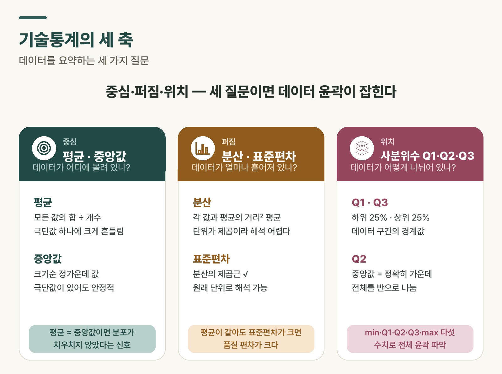 Figure 1. The three questions of descriptive statistics, and the measures for each
First question: where is the data clustered
Mean
The measure that comes to mind first. Add up every value and divide by the count.
For example, if 5 quote requests took 3, 4, 5, 4, and 14 days to complete, the mean is (3+4+5+4+14) ÷ 5 = 6.0 days.
It’s intuitive and easy to compute, but it has one fatal weakness: it’s sensitive to extreme values. That single 14-day case pulled the overall mean up by a full 2 days, even though the other 4 cases were all 5 days or less.
Median
The value sitting exactly in the middle once the data is sorted by size. Sort 3, 4, 4, 5, 14, and the middle value is 4. The mean (6.0) and the median (4.0) differ by a full 2 days.
💡 Key point: When the mean and median differ substantially, it’s a signal the data is skewed to one side. In that case, looking only at the mean gives you a distorted picture. This is covered in more depth with a real-world example in the mean trap post.
In practice: if you’re managing a KPI using the mean alone, get in the habit of checking the median alongside it. If the two are close, that’s reassuring; if they diverge sharply, that’s a signal to dig deeper into the data.
Second question: how spread out is the data
Even with the same mean, two datasets can behave completely differently. Team A and Team B might both average a 5-day lead time, but Team A might reliably finish every job in 4–6 days, while Team B swings wildly — some jobs done in 1 day, others taking 9. Spread measures capture that difference.
Variance
A number that captures how far each data point sits from the mean. Calculated like this:
- Subtract the mean from each value (deviation)
- Square each deviation (so negatives disappear)
- Average the squared values
For 3, 4, 4, 5, 14: the deviations from the mean of 6.0 are −3, −2, −2, −1, 8. Squared, that’s 9, 4, 4, 1, 64. The average of those is 16.4.
The problem is that the unit becomes “days²,” which is hard to interpret intuitively.
Standard deviation
The square root of variance. √16.4 ≈ 4.0 days. Because the unit returns to its original form, you can read it intuitively as “on average, about 4 days away from the mean.”
A large standard deviation means the data isn’t clustered evenly around the mean — it’s also a signal of low predictability.
In practice: if two suppliers have the same average lead time, compare their standard deviations. The one with the smaller standard deviation is the more predictable, stable supplier — information you’d miss by looking at the mean alone.
Third question: how is the data divided up
Quartiles
Boundary values that split data, sorted by size, into four equal parts.
- Q1 (first quartile): the boundary of the bottom 25%. 25% of the data falls below this value.
- Q2 (second quartile): same as the median. Exactly half the data falls below this value.
- Q3 (third quartile): the boundary of the top 25%. 75% of the data falls below this value.
For 3, 4, 4, 5, 14: Q1=4, Q2=4, Q3=5.
The five-number summary
Minimum, Q1, Q2 (median), Q3, and maximum — put these five numbers together, and you can grasp the full shape of a dataset at a glance.
| Min | Q1 | Q2 (median) | Q3 | Max | |
|---|---|---|---|---|---|
| Quote lead time | 3 days | 4 days | 4 days | 5 days | 14 days |
Table 1. Five-number summary of quote lead times
The gap between Q3 and Q1 (5–4=1) is called the IQR (interquartile range). IQR is also used as a rule of thumb for spotting outliers — values above Q3 + 1.5×IQR, or below Q1 − 1.5×IQR, are generally flagged as outlier candidates.
⚠️ Note: An outlier isn’t something to remove automatically. First figure out whether it belongs to a structurally different group — like outsourced procurement — or whether it’s simply a data entry error.
In practice: pull a regular five-number summary for production lead time or inventory quantity data. If the gap between the maximum and Q3 is unusually wide, that range likely contains data that needs an explanation.
Rabbit’s Takeaway
Learning descriptive statistics for the first time tends to become an exercise in memorizing formulas — the variance formula, the standard deviation formula. But what actually matters more is knowing what each measure is “trying to show you.”
The mean looks at the center. Standard deviation looks at the spread. Quartiles look at the shape of the distribution. Look at all three together, and hundreds of numbers compress into a few lines.
At work, I’ve been gradually shifting away from looking at just the mean when I check KPI numbers — checking the median, checking whether the standard deviation is large. Looking at the same data, but starting to see different things. That’s the first change learning descriptive statistics gave me. 😎
Read more