Making SAP data work properly in Excel: from Power Query to pivot tables

Hi, this is Rabbit! 🐰

You’ve probably had this experience: you export data from SAP into Excel, and values that look like numbers are left-aligned, filters don’t work right, and a pivot table you build comes back with sums of zero. They’re clearly numbers, but Excel is reading them as text.

SAP exports and Excel don’t get along well. There’s a reason you can’t just paste and go, and the tool that fixes it is Power Query.

Why SAP exports don’t work in Excel out of the box

SAP is an ERP system; Excel is a spreadsheet. Because the two handle data differently, files exported from SAP come loaded with things Excel doesn’t like.

The most common issue in SAP exports is “numbers stored as text.” If SUM returns 0, or a pivot table’s totals look off, this is the first thing to suspect.

Two-row headers are also common. Excel pivot tables expect a single header row to work properly. With two rows, a pivot either reads only the first row as the header, or throws an error outright.

Subtotal and total rows mixed into the middle of the data are another problem. If a “total” row gets treated like a regular data row, aggregation double-counts it and inflates the numbers. Empty cells with missing values are common too — especially when the same material code spans multiple rows, with the code only filled in on the first row and the rest left blank.

⚠️ Note: Fixing these issues by hand every time is a waste of time — you’ll be doing the exact same thing again next month with the same kind of data. Building a cleanup routine once in Power Query is the answer.

Cleaning it all up at once with Power Query

Power Query is a data preprocessing tool built into Excel. No separate installation needed — start from the top menu with Data → Get Data → From File.

Power Query’s core advantage is that it records your steps. Save a sequence like “convert this column to numbers, delete row 3, fill blank cells with the value above” and the next time you load a new file, the same steps run automatically. One click of Refresh, and you’re done.

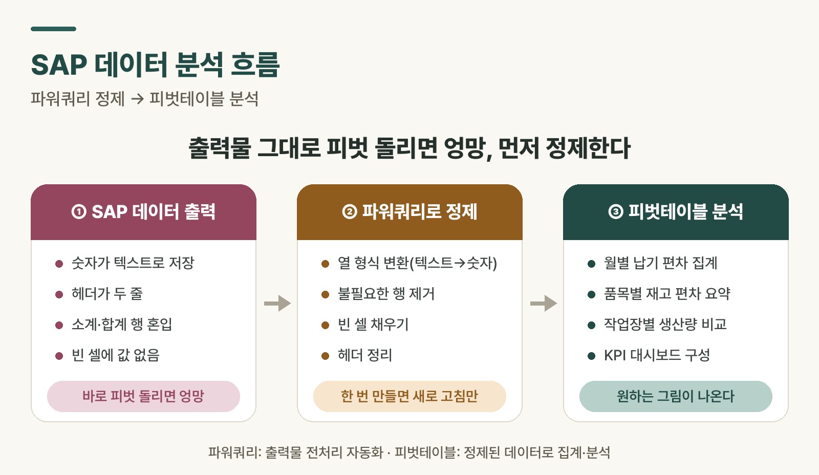Figure 1. Three-step flow: SAP export → Power Query cleanup → pivot analysis

The main cleanup steps are these:

Converting column types is the most basic step. Select the column of numbers stored as text and choose “Change Type → Whole Number” or “Decimal Number.” Set it up once, and it converts automatically every time after that.

Removing unwanted rows filters out subtotal and total rows. Use “Filter Rows → does not contain” to remove rows containing “Total” or “Subtotal.”

Filling blank cells handles cases like material codes, where only the first row in a block has a value and the rest are blank. Select the column and choose “Fill → Down” to copy the value above down through the blanks.

Cleaning up headers turns a two-row header into one row — either by removing the unneeded first row, or using the “Use First Row as Headers” option.

Analyzing with pivot tables

Data cleaned in Power Query connects straight into a pivot table. When inserting a pivot table, choosing “Add this data to the Data Model” lets you use the Power Query output directly.

For monthly delivery variance aggregation, put “month” in Rows and “average delivery variance” in Values, and the monthly trend appears immediately. Take the variance data covered in the inventory variance post and run it through a pivot, and you can see the distribution by item and by month at a glance.

For an inventory variance summary, put “material code” in Rows and “total variance” plus “variance count” in Values, and the scale of variance by item comes into focus. It becomes immediately obvious which items have the largest variance.

A pivot table is an exploration tool. It summarizes numbers and surfaces patterns, but figuring out why a pattern exists takes domain knowledge. When something odd shows up in a pivot, the next step — as covered in the correlation vs. causation post — is tracking down the cause behind the number.

Rabbit’s Takeaway

If you’ve got a routine of pulling SAP data into Excel, fixing it by hand, running a pivot, and starting the whole thing over again next month, Power Query can break that cycle in one move.

The first setup might take 30 minutes, but every month after that, it’s just a refresh. Automating repetitive work is the first step toward freeing up time for actual analysis. Cut down the time spent cleaning data, and the time spent reading it goes up. 😎

---

Read more

• Inventory variance: when the numbers check out but the floor doesn’t
• Descriptive statistics: the first thing you do when you face a new dataset