
Inventory variance: when the numbers check out but the floor doesn't
When SAP inventory and physical count don't match, here's how to read the variance statistically and track down the cause in practice.
Hi, this is Rabbit! 🐰
Physical inventory counts come around twice a year. The first-half count is mostly an internal check, but the second half is different — it feeds into the accounting audit, so every single variance number gets scrutinized closely. Put together audit response materials, and you’ll inevitably hit a moment where you have to explain “why is the variance on this item so large.”
Run a physical count, and this always happens: SAP says 100, but the actual count comes to 98. Or the opposite — you expected only 87, but the warehouse actually has 95. Whether the gap is big or small, a mismatch means something went missing somewhere along the way.
This gap is called inventory variance. Looking at variance item by item, though, gives you a completely different picture than summarizing it statistically. Let’s talk through that difference today.
- Inventory variance (physical count − SAP) matters in both direction (positive/negative) and magnitude.
- Average variance shows the overall direction; standard deviation shows how erratic it is.
- Variance generally comes from one of three causes — missed goods movements, defect handling errors, or data entry mistakes.
What is inventory variance
Inventory variance is simple: physical count − SAP quantity.
- Positive (+): the physical count is higher. SAP is under-recording inventory.
- Negative (−): the physical count is lower. SAP is over-recording inventory.
- 0: a match. The ideal state.
The real question is how to summarize variance when you’re dealing with hundreds or thousands of items. Look at each item one at a time, and no pattern emerges. This is where descriptive statistics comes in.
Reading variance statistically
Say a physical count for 5 items comes back like this.
| Item | SAP quantity | Physical count | Variance |
|---|---|---|---|
| Material A | 100 | 98 | −2 |
| Material B | 200 | 195 | −5 |
| Material C | 150 | 163 | +13 |
| Material D | 80 | 80 | 0 |
| Material E | 300 | 287 | −13 |
Table 1. Example of per-item inventory variance
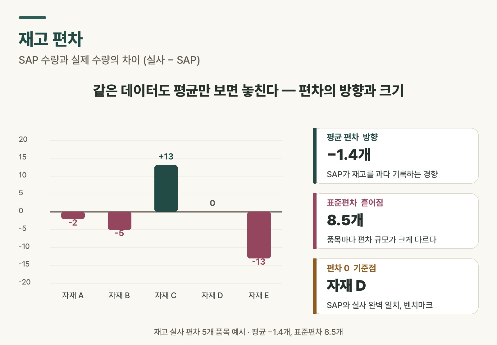 Figure 1. Distribution of per-item inventory variance — teal is physical-count surplus, berry is physical-count shortfall
Average variance — reading the overall direction
The average of the 5 variances is (−2 + −5 + 13 + 0 + −13) ÷ 5 = −1.4.
That’s negative — an overall skew toward the physical count coming in lower than SAP. A signal that SAP is recording more inventory than actually exists.
💡 Key point: An average variance close to 0 means things are broadly balanced overall. A large negative average suggests the system tends to over-record inventory; a large positive average suggests it tends to under-record.
Standard deviation — reading how erratic it is
The standard deviation of those 5 variances is about 8.5 — quite large relative to the average variance (−1.4).
What that means: the scale of variance differs wildly from item to item. Some are 0, some are +13, some are −13. The average alone tells you “off by about 1.4 units,” but the standard deviation reveals that “some individual items are actually off by more than 10.”
If the average variance is small but the standard deviation is large, positives and negatives are canceling each other out. The situation on the floor could be far messier than it looks.
In practice: managing overall inventory variance rate as a single (±) KPI can create an optical illusion. Looking at standard deviation or mean absolute deviation (MAD) alongside it gives a more accurate picture of the actual chaos.
Explaining variance during an accounting audit
The second-half physical count ties directly into the accounting audit. Auditors will ask for an explanation of any item with large variance. “We counted it and it was different” doesn’t cut it as an answer.
This is where statistically organized variance data earns its keep. Present the average variance and standard deviation together, and you can objectively show “which direction things are skewed, overall, and how spread out.” Pair items with large variance with their likely cause — missed goods movement, defect handling error, and so on.
💡 Key point: The core of audit response isn’t the size of the number — it’s explainability. Even if variance exists, having a known cause and a plan to prevent recurrence is itself evidence that internal controls are working.
Three causes behind variance
Once you’ve used statistics to pin down the scale and direction of variance, the next step is the cause. Inventory variance almost always comes from one of three sources.
First, missed goods movements. Something physically moved in or out of the warehouse, but no matching document got created in SAP. This is the most common cause — forgetting to issue material after it went into production, or a return that came in but never got processed as a receipt in time.
Second, errors in defect or scrap handling. A defect occurs, the physical unit gets quarantined in a corner of the warehouse, but it never gets scrapped in SAP. A physical count finds the quantity sitting in the quarantine area, and SAP still shows that same quantity as available. The variance looks like zero, but the actual usable inventory is different.
Third, data entry mistakes. Entering the wrong quantity or confusing units — entering 10 boxes as 10 units, for example.
⚠️ Note: Before chasing the cause of a variance, first figure out whether “this is a counting error, or a process problem.” A miscount during the physical inventory and an unprocessed goods issue during normal operations call for completely different fixes.
Learning from the items with zero variance
Material D has zero variance. SAP quantity and physical count match exactly.
That might seem too simple to matter, but it could be the most important data point of all. An item with zero variance means its goods movement process is working well. Look at how that item’s owner manages it, what process they follow, and applying the same approach to other items becomes a lead for reducing overall variance.
In variance analysis, it’s important to look not just at “what went wrong” but also at “what went right.”
In practice: as covered in the descriptive statistics concept note, looking at variance distribution through quartiles alongside the mean and standard deviation enables more precise analysis. Find what the bottom 25% (Q1) of items with the smallest variance have in common, and you can identify the conditions behind good management.
Rabbit’s Takeaway
Once a physical inventory count wraps up, it usually ends with just a number: “this many were off.” But gather those numbers up and compute the average and standard deviation, and a completely different story emerges.
Is there an overall skew in the negative direction? How erratic is the variance from item to item? Knowing that makes it far clearer where to start fixing things. Chasing every single variance one by one is far less efficient than reading the pattern statistically first and narrowing down the cause from there.
Turning “the inventory doesn’t add up” from a gut feeling into something you can say with numbers — that’s why I’m studying statistics right now. 😎
Read more